Binning transformer

Demonstrates how to bin continuous features in your dataset.

Out:

a  ...      b_binned
0  5.1  ...  (3.30, 3.90]
1  4.9  ...  (2.70, 3.30]
2  4.7  ...  (2.70, 3.30]
3  4.6  ...  (2.70, 3.30]
4  5.0  ...  (3.30, 3.90]

[5 rows x 6 columns]

print(__doc__)

# Author: Taylor Smith <taylor.smith@alkaline-ml.com>

from matplotlib import pyplot as plt
from skoot.datasets import load_iris_df
from skoot.preprocessing import BinningTransformer

# #############################################################################
# load data
iris = load_iris_df(include_tgt=False, names=["a", "b", "c", "d"])
binner = BinningTransformer(cols=["a", "b"], return_bin_label=True,
                            strategy="uniform", overwrite=False,
                            n_bins=4)

# print the head of the binned dataset
print(binner.fit_transform(iris).head())

# #############################################################################
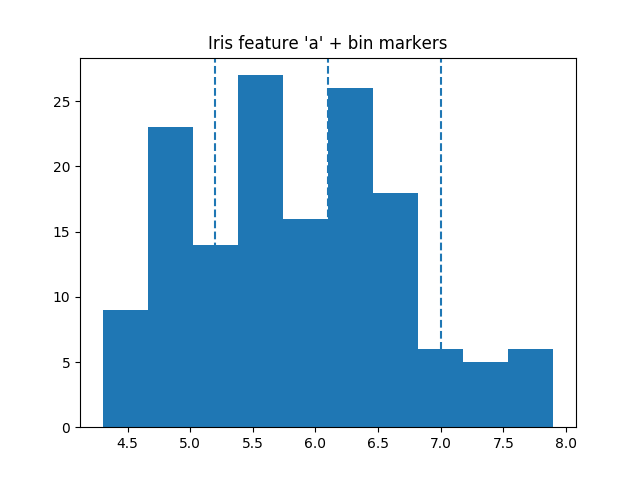
# Show where the boundaries reside

a_lower = binner.bins_["a"].lower_bounds[1:]  # skip the -np.inf
plt.hist(iris["a"].values)

# plot vertical lines where bins are
for bound in a_lower:
    plt.axvline(bound, ls="--")
plt.title("Iris feature 'a' + bin markers")
plt.show()

Total running time of the script: ( 0 minutes 0.059 seconds)